Electrodialysis (0D)
from watertap.unit_models.electrodialysis_0D import Electrodialysis0D
Introduction
Electrodialysis, an electrochemical separation technology, has been utilized to desalinate water for decades. Compared with other technologies, such as reverse osmosis (RO), electrodialysis shows advantages in desalinating brackish waters with moderate salinity by its less intense energy consumption, higher water recovery, and robust tolerance for adverse non-ionic components (e.g., silica and biological substances) in water. Between the electrodes of an electrodialysis stack (a reactor module), multiple anion- and cation-exchange membranes are alternately positioned and separated by spacers to form individual cells. When operated, electrodialysis converts electrical current to ion flux and, assisted by the opposite ion selectivity of cation- and anion-exchange membranes (cem and aem), moves ion from one cell to its adjacent cell in a cell-pair treatment unit (Figure 1). The ion-departing cell is called a diluate channel and the ion-entering cell a concentrate channel. Recovered (desalinated) water is collected from diluate channles of all cell pairs while the concentrate product can be disposed of as brine or retreated. More overview of the electrodialysis technology can be found in the References.
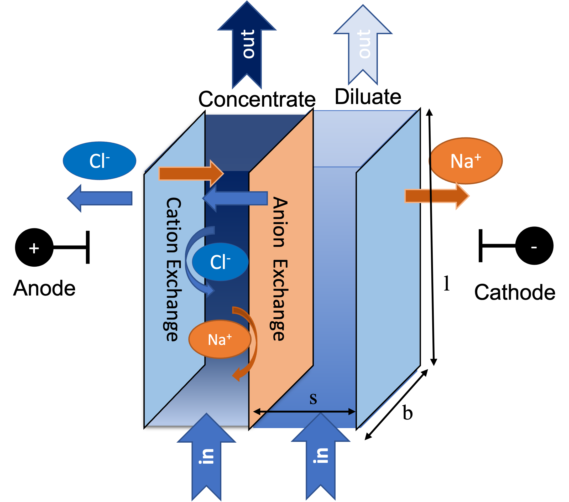
Figure 1. Schematic representation of an electrodialysis cell pair
One cell pair in an electrodialysis stack can thus be treated as a modeling unit that can multiply to larger-scale systems. The presented electrodialysis model establishes mathematical descriptions of ion and water transport in a cell pair and expands to simulate a stack with a specified cell-pair number. Modeled mass transfer mechanisms include electrical migration and diffusion of ions and osmosis and electroosmosis of water. The following key assumptions are based on.
The concentrate and diluate channels have identical geometry.
For each channel, component fluxes are uniform in the bulk solutions (the 0-dimensional assumption) and are set as the average of inlet and outlet of each channel.
Steady state: all variables are independent on time.
Co-current flow operation.
Electrical current is operated below the limiting current.
Ideality assumptions: activity, osmotic, and van’t Hoff coefficients are set at one.
All ion-exchange membrane properties (ion and water transport number, resistance, permeability) are constant.
Detailed concentration gradient effect at membrane-water interfaces is neglected.
Constant pressure and temperature through each channel.
Control Volumes
This model has two control volumes for the concentrate and diluate channels.
Diluate
Concentrate
Ports
On the two control volumes, this model provides four ports (Pyomo notation in parenthesis):
inlet_diluate (inlet)
outlet_diluate (outlet)
inlet_concentrate (inlet)
outlet_concentrate (outlet)
Sets
This model can simulate the electrodialysis desalination of a water solution containing multiple species (neutral or ionic). All solution components ( H2O, neutral solutes, and ions) form a Pyomo set in the model. For a clear model demonstration, this document uses a NaCl water solution as an instance hereafter.
This model can mathematically take a multi-component (i.e., > one salt molecule to be treated) as an input; nevertheless a multi-component solution creates unknown or difficult-to-specify parameters, e.g., the electrical transport numbers through membranes, the multi-ion diffusivity, etc., and physical relationships, which may result in ill-posed or ill-conditioned problems challenging the models’ numerical solutions. While we continuously work on advancing our models to absorb new principles revealed by progressing research, we advise the users be very cautious with simulating multi-component systems by this programmed model for aspects stated above.
Description |
Symbol |
Indices |
|---|---|---|
Time |
\(t\) |
[t] ([0])1 |
Phase |
\(p\) |
[‘Liq’] |
Component |
\(j\) |
[‘H2O’, ‘Na_+’, ‘Cl_-‘] |
Ion |
\(j\) |
[‘Na_+’, ‘Cl_-’] 2 |
Membrane |
n/a |
[‘cem’, ‘aem’] |
- Notes
1 The time set index is set as [0] in this steady-state model and is reserved majorly for the future extension to a dynamic model.
2 “Ion” is a subset of “Component” and uses the same symbol j.
Degrees of Freedom
Applying this model to a NaCl solution yields 33 degrees of freedom (Table 2), among which temperature, pressure, and component molar flow rate are state variables that are fixed as initial conditions. The rest are parameters that should be provided in order to fully solve the model.
Description |
Symbol |
Variable Name |
Index |
Units |
DOF Number 1 |
|---|---|---|---|---|---|
Temperature, inlet_diluate |
\(T^D\) |
temperature |
None |
\(K\) |
1 |
Temperature, inlet_concentrate |
\(T^C\) |
temperature |
None |
\(K\) |
1 |
Pressure, inlet_diluate |
\(p^D\) |
temperature |
None |
\(Pa\) |
1 |
Pressure, inlet_concentrate |
\(p^C\) |
temperature |
None |
\(Pa\) |
1 |
Component molar flow rate, inlet_diluate |
\(N_{j, in}^D\) |
flow_mol_phase_comp |
[t], [‘Liq’], [‘H2O’, ‘Na_+’, ‘Cl_-‘] |
\(mol s^{-1}\) |
3 |
Component molar flow rate, inlet_concentrate |
\(N_{j, in}^C\) |
flow_mol_phase_comp |
[t], [‘Liq’], [‘H2O’, ‘Na_+’, ‘Cl_-‘] |
\(mol s^{-1}\) |
3 |
Water transport number |
\(t_w\) |
water_trans_number_membrane |
[‘cem’, ‘aem’] |
dimensionless |
2 |
Water permeability |
\(L\) |
water_permeability_membrane |
[‘cem’, ‘aem’] |
\(m^{-1}s^{-1}Pa^{-1}\) |
2 |
Voltage or Current 2 |
\(U\) or \(I\) |
voltage or current |
[t] |
\(\text{V}\) or \(A\) |
1 |
Electrode areal resistance |
\(r_{el}\) |
electrodes_resistance |
[t] |
\(\Omega m^2\) |
1 |
Cell pair number |
\(n\) |
cell_pair_num |
None |
dimensionless |
1 |
Current utilization coefficient |
\(\xi\) |
current_utilization |
None |
dimensionless |
1 |
Spacer thickness |
\(s\) |
spacer_thickness |
none |
\(m\) |
1 |
Membrane areal resistance |
\(r\) |
membrane_surface_resistance |
[‘cem’, ‘aem’] |
\(\Omega m^2\) |
2 |
Cell width |
\(b\) |
cell_width |
None |
\(\text{m}\) |
1 |
Cell length |
\(l\) |
cell_length |
None |
\(\text{m}\) |
1 |
Thickness of ion exchange membranes |
\(\delta\) |
membrane_thickness |
[‘cem’, ‘aem’] |
\(m\) |
2 |
diffusivity of solute in the membrane phase |
\(D\) |
solute_diffusivity_membrane |
[‘cem’, ‘aem’], [‘Na_+’, ‘Cl_-‘] |
\(m^2 s^{-1}\) |
4 |
transport number of ions in the membrane phase |
\(t_j\) |
ion_trans_number_membrane |
[‘cem’, ‘aem’], [‘Na_+’, ‘Cl_-‘] |
dimensionless |
4 |
- Note
1 DOF number takes account of the indices of the corresponding parameter.
2 A user should provide either current or voltage as the electrical input, in correspondence to the “Constant_Current” or “Constant_Voltage” treatment mode (configured in this model). The user also should provide an electrical magnitude that ensures a operational current below the limiting current of the feed solution.
Solution component information
To fully construct solution properties, users need to provide basic component information of the feed solution to use this model, including identity of all solute species (i.e., Na +, and Cl - for a NaCl solution), molecular weight of all component species (i.e., H2O, Na +, and Cl -), and charge and electrical mobility of all ionic species (i.e., Na +, and Cl -). This can be provided as a solution dictionary in the following format (instanced by a NaCl solution).
ion_dict = {
         "solute_list": ["Na_+", "Cl_-"],
         "mw_data": {"H2O": 18e-3, "Na_+": 23e-3, "Cl_-": 35.5e-3},
         "electrical_mobility_data": {"Na_+": 5.19e-8, "Cl_-": 7.92e-8},
         "charge": {"Na_+": 1, "Cl_-": -1},
     }
This model, by default, uses H2O as the solvent of the feed solution.
Information regarding the property package this unit model relies on can be found here:
watertap.property_models.ion_DSPMDE_prop_pack
Equations
This model solves mass balances of all solution components (H2O, Na +, and Cl - for a NaCl solution) on two control volumes (concentrate and diluate channels). Mass balance equations are summarized in Table 3. Mass transfer mechanisms take account of solute electrical migration and diffusion and water osmosis and electroosmosis. Theoretical principles, e.g., continuity equation, Fick’s law, and Ohm’s law, to simulate these processes are well developed and some good summaries for the electrodialysis scenario can be found in the References.
Description |
Equation |
Index set |
|---|---|---|
Component mass balance |
\(N_{j, in}^{C\: or\: D}-N_{j, out}^{C\: or\: D}+J_j^{C\: or\: D} bl=0\) |
\(j \in \left['H_2 O', '{Na^{+}} ', '{Cl^{-}} '\right]\) |
mass transfer flux, concentrate, solute |
\(J_j^{C} = \left(t_j^{cem}-t_j^{aem} \right)\frac{\xi i}{ z_j F}-\left(\frac{D_j^{cem}}{\delta ^{cem}} +\frac{D_j^{aem}}{\delta ^{aem}}\right)\left(c_j^C-c_j^D \right)\) |
\(j \in \left['{Na^{+}} ', '{Cl^{-}} '\right]\) |
mass transfer flux, diluate, solute |
\(J_j^{D} = -\left(t_j^{cem}-t_j^{aem} \right)\frac{\xi i}{ z_j F}+\left(\frac{D_j^{cem}}{\delta ^{cem}} +\frac{D_j^{aem}}{\delta ^{aem}}\right)\left(c_j^C-c_j^D \right)\) |
\(j \in \left['{Na^{+}} ', '{Cl^{-}} '\right]\) |
mass transfer flux, concentrate, H2O |
\(J_j^{C} = \left(t_w^{cem}+t_w^{aem} \right)\left(\frac{i}{F}\right)+\left(L^{cem}+L^{aem} \right)\left(p_{osm}^C-p_{osm}^D \right)\left(\frac{\rho_w}{M_w}\right)\) |
\(j \in \left['H_2 O'\right]\) |
mass transfer flux, diluate, H2O |
\(J_j^{D} = -\left(t_w^{cem}+t_w^{aem} \right)\left(\frac{i}{F}\right)-\left(L^{cem}+L^{aem} \right)\left(p_{osm}^C-p_{osm}^D \right)\left(\frac{\rho_w}{M_w}\right)`\) |
\(j \in \left['H_2 O'\right]\) |
Additionally, several other equations are built to describe the electrochemical principles and electrodialysis performance.
Description |
Equation |
|---|---|
Current density |
\(i = \frac{I}{bl}\) |
Ohm’s Law |
\(U = i r_{tot}\) |
Resistance calculation |
\(r_{tot}=n\left(r^{cem}+r^{aem}+\frac{d}{\kappa^C}+\frac{d}{\kappa^D}\right)+r_{el}\) |
Electrical power consumption |
\(P=UI\) |
Water-production-specific power consumption |
\(P_Q=\frac{UI}{3.6\times 10^6 nQ_{out}^D}\) |
Overall current efficiency |
\(I\eta=\sum_{j \in[cation]}{\left[\left(N_{j,in}^D-N_{j,out}^D\right)z_j F\right]}\) |
All equations are coded as “constraints” (Pyomo). Isothermal and isobaric conditions apply.
Extended simulation
This model supports extensive simulations of (1) the nonohmic potential across ion exchange membranes and (2) the Nernst diffusion layer. Users can customize these extenions via two configurations: has_nonohmic_potential_membrane that triggers the calculation of nonohmic potentials across ion exchange membranes and has_Nernst_diffusion_layer that triggers the simulation of a concentration-polarized Nernst diffusion layer including its ohmic and nonohmic potential changes. Based on a electrochemical cell setup in Figure 2 and established theoretical descriptions (References), our model accounts for the cross-membrane diffusion and Donnan potentials (nonohmic), ion concentration polarization in assumed Nernst diffusion layers (NDL), and the ohmic and nonohmic (i.e., diffusion) potentials across NDLs. These extensions make the model closer to the non-ideal physical conditions that can be encountered in real desalination practices.
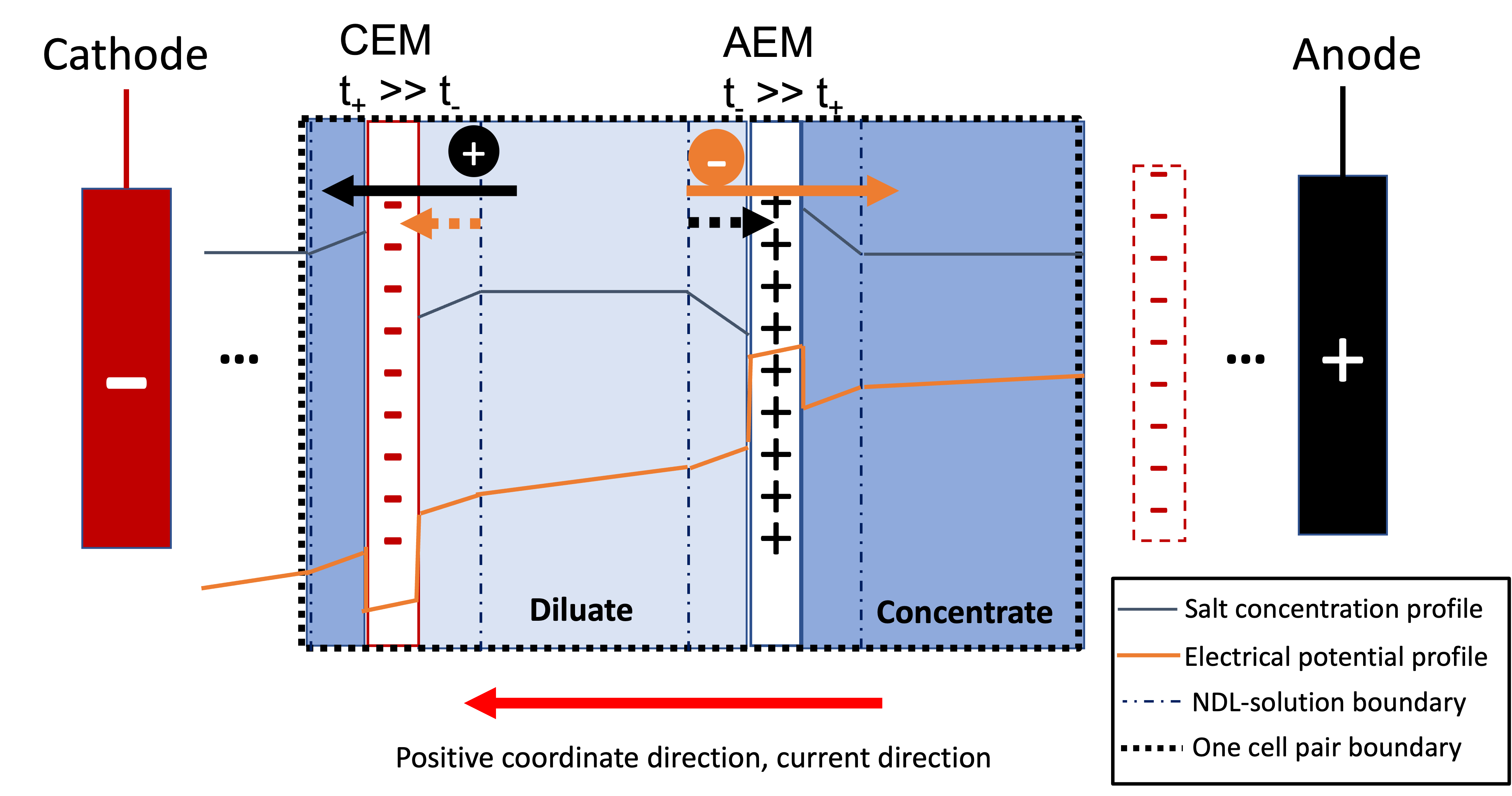
Figure 2. Electrochemical cell setup for simulating Nernst diffusion layer and cross-membrane potential and concentration variations.
Table 5 presents the equations underlying the two extensions assuming a 1:1 symmetric electrolyte such as NaCl.
Description |
Equation |
Condition |
|---|---|---|
Limiting current density |
\(i_{lim} = i_{lim,0}\frac{c^D}{c^D_{in}}\) |
has_Nernst_diffusion_layer==True and limiting_current_density_method == LimitingCurrentDensityMethod.InitialValue |
\(i_{lim} = A v^B c^D\) |
has_Nernst_diffusion_layer==True and limiting_current_density_method == LimitingCurrentDensityMethod.Empirical |
|
\(i_{lim} = \frac{Sh F D_b c^D}{d_H \left(t_+^{cem}-t_+ \right)}\) |
has_Nernst_diffusion_layer==True and limiting_current_density_method == LimitingCurrentDensityMethod.Theoretical |
|
Nonohmic potential, membrane |
\(\phi_m=\frac{RT}{F} \left( t_+^{iem} - t_-^{iem} \right) \ln \left( \frac{c_s^R}{c_s^L} \right)\) |
has_nonohmic_potential_membrane == True |
Ohmic potential, NDL |
\(\phi_d^{ohm}=\frac{FD_b}{\left(t_+^{iem}-t_+\right)\lambda}\ln\left(\frac{c_s^Lc_b^R}{c_s^Rc_b^L}\right)\) |
has_Nernst_diffusion_layer==True |
Nonohmic potential, NDL |
\(\phi_d^{nonohm}=\frac{RT}{F}\left(t_+-t_-\right) \ln\left(\frac{c_s^Lc_b^R}{c_s^Rc_b^L}\right)\) |
has_Nernst_diffusion_layer==True |
NDL thickness, cem |
\(\Delta^{L/R} = \frac{F D_b c_b^{L/R}}{\left(t_+^{iem}-t_+ \right) i_{lim}}\) |
has_Nernst_diffusion_layer==True |
NDL thickness, aem |
\(\Delta^{L/R} = - \frac{F D_b c_b^{L/R}}{\left(t_+^{iem}-t_+\right) i_{lim}}\) |
has_Nernst_diffusion_layer==True |
Concentration polarization ratio, cem |
\(\frac{c_s^L}{c_b^L} = 1+\frac{i}{i_{lim}},\qquad \frac{c_s^R}{c_b^R} = 1-\frac{i}{i_{lim}}\) |
has_Nernst_diffusion_layer==True 1 |
Concentration polarization ratio, aem |
\(\frac{c_s^L}{c_b^L} = 1-\frac{i}{i_{lim}},\qquad \frac{c_s^R}{c_b^R} = 1+\frac{i}{i_{lim}}\) |
has_Nernst_diffusion_layer==True |
Note
1 When this configuration is turned off, \(i_{lim}\) is considered as \(\infty\) and the ratio becomes 1.
Some other modifications to previously defined equations are made to accommodate the two extensions. These are shown in Table 6.
Original equation description |
Equation replacement |
Condition |
|---|---|---|
Ohm’s law |
\(u = i r_{tot} + \phi_m + \phi_d^{ohm} + \phi_d^{nonohm}\) 1 |
has_nonohmic_potential_membrane == True and/or has_Nernst_diffusion_layer==True |
Resistance calculation |
\(r_{tot}=n\left(r^{cem}+r^{aem}+\frac{d- \Delta_{cem}^L - \Delta_{aem}^R}{\kappa^C}+\frac{d- \Delta_{cem}^R - \Delta_{aem}^L}{\kappa^D}\right)+r_{el}\) |
has_Nernst_diffusion_layer==True |
mass transfer flux, concentrate, solute |
\(J_j^{C} = \left(t_j^{cem}-t_j^{aem} \right)\frac{\xi i}{ z_j F}-\left(\frac{D_j^{cem}}{\delta ^{cem}}\left(c_{s,j}^{L,cem}-c_{s,j}^{R,cem} \right) +\frac{D_j^{aem}}{\delta ^{aem}} \left(c_{s,j}^{R,aem}-c_{s,j}^{L,aem} \right)\right)\) |
has_nonohmic_potential_membrane == True and/or has_Nernst_diffusion_layer==True |
mass transfer flux, diluate, solute |
\(J_j^{D} = -\left(t_j^{cem}-t_j^{aem} \right)\frac{\xi i}{ z_j F}+\left(\frac{D_j^{cem}}{\delta ^{cem}}\left(c_{s,j}^{L,cem}-c_{s,j}^{R,cem} \right) +\frac{D_j^{aem}}{\delta ^{aem}} \left(c_{s,j}^{R,aem}-c_{s,j}^{L,aem} \right)\right)\) |
has_nonohmic_potential_membrane == True and/or has_Nernst_diffusion_layer==True |
mass transfer flux, concentrate, H2O |
\(J_j^{C} = \left(t_w^{cem}+t_w^{aem} \right)\frac{i}{F}+\left(L^{cem} \left(p_{s, osm}^{cem, L}-p_{s, osm}^{cem, R} \right)+L^{aem} \left(p_{s, osm}^{aem, R}-p_{s, osm}^{aem, L} \right)\right)\frac{\rho_w}{M_w}\) |
has_Nernst_diffusion_layer==True |
mass transfer flux, diluate, H2O |
\(J_j^{D} = -\left(t_w^{cem}+t_w^{aem} \right)\frac{i}{F}-\left(L^{cem} \left(p_{s, osm}^{cem, L}-p_{s, osm}^{cem, R} \right)+L^{aem} \left(p_{s, osm}^{aem, R}-p_{s, osm}^{aem, L} \right)\right)\frac{\rho_w}{M_w}\) |
has_Nernst_diffusion_layer==True |
Note
1 \(\phi_m, \phi_d^{ohm}\) or \(\phi_d^{nonohm}\) takes 0 if its corresponding configuration is turned off (value == False).
Frictional pressure drop
This model can optionally calculate pressured drops along the flow path in the diluate and concentrate channels through config has_pressure_change and pressure_drop_method. Under the assumption of identical diluate and concentrate channels and starting flow rates, the flow velocities in the two channels are approximated equal and invariant over the channel length when calculating the frictional pressure drops. This approximation is based on the evaluation that the actual velocity variation over the channel length caused by water mass transfer across the consecutive channels leads to negligible errors as compared to the uncertainties carried by the frictional pressure method itself. Table 7 gives essential equations to simulate the pressure drop. Among extensive literatures using these equations, a good reference paper is by Wright et. al., 2018 (References).
Description |
Equation |
Condition |
|---|---|---|
Frictional pressure drop, Darcy_Weisbach |
\(p_L=f\frac{\rho v^2}{2d_H}\) 1 |
has_pressure_change == True and pressure_drop_method == PressureDropMethod.Darcy_Weisbach |
\(p_L=\) user-input constant |
has_pressure_change == True and pressure_drop_method == PressureDropMethod.Experimental |
|
Hydraulic diameter |
\(d_H=\frac{2db(1-\epsilon)}{d+b}\) |
hydraulic_diameter_method == HydraulicDiameterMethod.conventional |
\(d_H=\frac{4\epsilon}{\frac{2}{h}+(1-\epsilon)S_{v,sp}}\) |
hydraulic_diameter_method == HydraulicDiameterMethod.spacer_specific_area_known |
|
Renold number |
\(Re=\frac{\rho v d_H}{\mu}\) |
has_pressure_change == True or limiting_current_density_method == LimitingCurrentDensityMethod.Theoretical |
Schmidt number |
\(Sc=\frac{\mu}{\rho D_b}\) |
has_pressure_change == True or limiting_current_density_method == LimitingCurrentDensityMethod.Theoretical |
Sherwood number |
\(Sh=0.29Re^{0.5}Sc^{0.33}\) |
has_pressure_change == True or limiting_current_density_method == LimitingCurrentDensityMethod.Theoretical |
Darcy’s frictional factor |
\(f=4\times 50.6\epsilon^{-7.06}Re^{-1}\) |
friction_factor_method == FrictionFactorMethod.Gurreri |
\(f=4\times 9.6 \epsilon^{-1} Re^{-0.5}\) |
friction_factor_method == FrictionFactorMethod.Kuroda |
|
Pressure balance |
\(p_{in}-p_L l =p_{out}\) |
has_pressure_change == True |
Note
1 We assumed a constant linear velocity (in the cell length direction), \(v\), in both channels and along the flow path. This \(v\) is calculated based on the average of inlet and outlet volumetric flow rate.
Nomenclature
Symbol |
Description |
Unit |
|---|---|---|
Parameters |
||
\(\rho_w\) |
Mass density of water |
\(kg\ m^{-3}\) |
\(M_w\) |
Molecular weight of water |
\(kg\ mol^{-1}\) |
Variables and Parameters |
||
\(N\) |
Molar flow rate of a component |
\(mol\ s^{-1}\) |
\(J\) |
Molar flux of a component |
\(mol\ m^{-2}s^{-1}\) |
\(b\) |
Cell/membrane width |
\(m\) |
\(l\) |
Cell/membrane length |
\(m\) |
\(t\) |
Ion transport number |
dimensionless |
\(I\) |
Current |
\(A\) |
\(i\) |
Current density |
\(A m^{-2}\) |
\(U\) |
Voltage over a stack |
\(V\) |
\(n\) |
Cell pair number |
dimensionless |
\(\xi\) |
Current utilization coefficient (including ion diffusion and water electroosmosis) |
dimensionless |
\(z\) |
Ion charge |
dimensionless |
\(F\) |
Faraday constant |
\(C\ mol^{-1}\) |
\(D\) |
Ion Diffusivity |
\(m^2 s^{-1}\) |
\(\delta\) |
Membrane thickness |
\(m\) |
\(c\) |
Solute concentration |
\(mol\ m^{-3}\) |
\(t_w\) |
Water electroosmotic transport number |
dimensionless |
\(L\) |
Water permeability (osmosis) |
\(ms^{-1}Pa^{-1}\) |
\(p_{osm}\) |
Osmotic pressure |
\(Pa\) |
\(r_{tot}\) |
Total areal resistance |
\(\Omega m^2\) |
\(r\) |
Membrane areal resistance |
\(\Omega m^2\) |
\(r_{el}\) |
Electrode areal resistance |
\(\Omega m^2\) |
\(d\) |
Spacer thickness |
\(m\) |
\(\kappa\) |
Solution conductivity |
\(S m^{-1}\ or\ \Omega^{-1} m^{-1}\) |
\(\eta\) |
Current efficiency for desalination |
dimensionless |
\(P\) |
Power consumption |
\(W\) |
\(P_Q\) |
Specific power consumption |
\(kW\ h\ m^{-3}\) |
\(Q\) |
Volume flow rate |
\(m^3s^{-1}\) |
\(\phi_m\) |
Nonohmic potential across a membrane |
\(V\) |
\(\phi_d^{ohm}\) |
Ohmic potential across a Nernst diffusion layer |
\(V\) |
\(\phi_d^{nonohm}\) |
Nonohmic potential across a Nernst diffusion layer |
\(V\) |
\(\Delta\) |
Nernst diffusion layer thickness |
\(m\) |
\(D_b\) |
Diffusivity of the salt molecular in the bulk solution |
\(m^2 s^{-1}\) |
\(i_{lim}\) |
Limiting current density |
\(A m^{-2}\) |
\(\lambda\) |
equivalent conductivity of the solution |
\(m^2 \Omega^{-1} mol^{-1}\) |
Subscripts and superscripts |
||
\(C\) |
Concentrate channel |
|
\(D\) |
Diluate channel |
|
\(j\) |
Component index |
|
\(in\) |
Inlet |
|
\(out\) |
Outlet |
|
\(cem\) |
Cation exchange membrane |
|
\(aem\) |
Anion exchange membrane |
|
\(iem\) |
Ion exchange membrane, i.e., cem or aem |
|
\(L\) |
The left side of a membrane, facing the cathode |
|
\(R\) |
The right side of a membrane, facing the anode |
|
\(s\) |
location of the membrane surface |
|
\(b\) |
location of bulk solution |
|
\(+\) or \(-\) |
mono-cation or mono-anion |
References
Strathmann, H. (2010). Electrodialysis, a mature technology with a multitude of new applications. Desalination, 264(3), 268-288.
Strathmann, H. (2004). Ion-exchange membrane separation processes. Elsevier. Ch. 4.
Campione, A., Cipollina, A., Bogle, I. D. L., Gurreri, L., Tamburini, A., Tedesco, M., & Micale, G. (2019). A hierarchical model for novel schemes of electrodialysis desalination. Desalination, 465, 79-93.
Campione, A., Gurreri, L., Ciofalo, M., Micale, G., Tamburini, A., & Cipollina, A. (2018). Electrodialysis for water desalination: A critical assessment of recent developments on process fundamentals, models and applications. Desalination, 434, 121-160.
Spiegler, K. S. (1971). Polarization at ion exchange membrane-solution interfaces. Desalination, 9(4), 367-385.
Wright, N. C., Shah, S. R., & Amrose, S. E. (2018). A robust model of brackish water electrodialysis desalination with experimental comparison at different size scales. Desalination, 443, 27-43.